Generative machine learning from a probabilistic perspective

Introduction

This article is my take on how the tools of probability can help us give a quantified meaning to the philosophical notion of causality. Modern probabilistic programming offers useful tools to uncover and quantify the different causes lying behind observations. We propose a short introduction to the field of probabilistic inference and how it underpins empirical results in different fields of pratical machine learning.

Formalism

We consider that our data are realizations of a random variable $x$, which is explained, at least partially, by a set of latent variables $z$. These latent variables act as causes for our observations but since, most of the time they cannot be observed, they must be infered from the data. This problem of probabilitic inference requires to encode our knowledge in a model $p$, which reflects the structure of causality.

For example, suppose we want to measure weight $w$ of an object but are only provided with an unreliable scale, which gives slightly different results for each measure. We are facing two different kinds of uncertainty: the one associated with the unknown weight and the one associated with the scale itself. Provided a first guess $g$, we can define the following probabilistic model.

\[\left\{ \begin{align} w & \mid g \sim \mathcal{N}(g, \sigma) \\ m & \mid g, w \sim \mathcal{N}(w, \tau) \end{align} \right.\]

The measurements $m$ are the only observed random variables, which are determined by the underlying weight, considered a latent cause, with its own uncertainty. Both uncertainties are modeled by Gaussian laws with standard deviations $\sigma$ and $\tau$ respectively. The parameters $\theta$ of the model correspond to constant scalars or vectors, here $\theta = \{g, \sigma, \tau\}$. Fitting the model means finding the optimal set $\theta^*$ according to a criterion, which is analogous to learning a model with respect to a given loss function in conventional machine learning.

Maximum likelihood criterion

We call evidence the probability of the data $x$ with respect to the model, simply denoted $p_\theta(x)$. The usual optimization criterion is to find the parameters $\theta$ such as the evidence of the data is maximal, therefore

\[\theta^* := \underset{\theta}{\operatorname{arg max}} p_\theta(x)\]

Linear regression

Linear regression is a simple model acting as a building block of deep learning models. We assume that the data are noisy observations of a linear combination of the latent variables $z$. With $w$ the weight vector to be fitted and a normal prior on the observation noise $\epsilon$, the model writes:

\[\left\{ \begin{align} x & = z w + \epsilon \\ \epsilon & \sim \mathcal{N}(0, \sigma^2) \end{align} \right.\]

Using the conditional probability notation, we have $x \mid z, w \sim \mathcal{N}(z w, \sigma^2)$. Therefore, the maximum likelihood estimator (MLE) on the parameters $\theta = \{w\}$ boils down to the usual mean squared error minimization rule (MSE). This is a direct consequence of the normality assumption.

\[\begin{align} \theta^* & := \underset{\theta}{\operatorname{arg max}} p_\theta(x \mid z, w) \\ & = \underset{w}{\operatorname{arg max}} \exp \left(- \lVert x - zw \rVert^2 / \sigma^2 \right) \\ & = \underset{w}{\operatorname{arg min}} \lVert x - zw \rVert^2 \end{align}\]

Ridge regression

To avoid overfitting the data, we usually add a regularizer on the parameter $w$, e.g. a Tikhonov regularizer $\lambda \lVert w \rVert^2$ to elastically control the weight dispersion. This is also explained by the MLE rule by further adding a normal prior on $w$.

\[\left\{ \begin{align} x & = z w + \epsilon \\ \epsilon & \sim \mathcal{N}(0, \sigma^2) \\ w &\sim \mathcal{N}(0, \tau^2) \end{align} \right.\]

By applying Bayes’ rule on the posterior $w \mid x,z$, we get $p(w \mid x,z) = p(x \mid z,w) \, p(w) \, / \, p(x \mid z)$ which leads to the usual ridge regression formulation:

\[w^* := \underset{w}{\operatorname{arg min}} \lVert x - zw \rVert^2 + \lambda \lVert w \rVert^2\]

Where $\lambda := \sigma^2 \, / \, \tau^2$. The MLE criterion enriched with a prior on the weight parameter is often refered as the maximum a posteriori rule (MAP) and underscores how regularization relates to structured uncertainty.

Unsupervised learning of the latent space

We now have a practical criterion to solve for the best $\theta$ given the uncertainty structure we associate with the problem. This rule concerns a supervised context, where we are provided with both $x$ and $z$ for training. In a more realistic setup, we only have $x$ observations to infer for the causes. It corresponds to inductive reasoning, where we try to infer the probables causes of observables effects.

The maching learning toolkit for this unsupervised learning includes autoencoders, a kind of network consisting of two symmetrical sub-networks:

• the encoder $p_\theta(x)$: learns the mapping from observations $x$ to latent variables $z$;
• the decoder $q_\phi(z)$: learns the inverse mapping, from the latent variables $z$ back to the observations $x$.

We train both simultaneously to reconstruct the observed variables through the latent space

\[\theta^*, \phi^* := \underset{\theta,\phi}{\operatorname{arg min}} \lVert x - (q_\phi \circ p_\theta) \, x \rVert^2\]

Variational inference

We consider the generic case of a graphical model $p_\theta$ with a hierarchy of latent variables $z$ and conditioning relations between them. The two problems of interest are:

• model fitting: selecting the best set of parameters $\theta^*$ with respect to the MLE criterion;
• posterior estimation: approximating the posterior distributions $p_{\theta^*}(z \mid x)$ for each $z$ given observed data $x$.

Applying the MLE criterion on the log-evidence, we get

\[\begin{align} \theta^* & := \underset{\theta}{\operatorname{arg max}} \log p_\theta(x) \\ & = \underset{\theta}{\operatorname{arg max}} \log \int_z p_\theta(x,z) \, dz \end{align}\]

The integral over the causes $z$ is often intractable and the associated optimization non-convex, making the whole problem especially strenuous to tackle. Furthermore, once $\theta^*$ is estimated, computing the prior also requires to approximate an intractable integral:

\[p_{\theta^*}(z \mid x) = \frac{p_{\theta^*}(x,y)}{\int p_{\theta^*}(x,z) \, dz}\]

Variational distribution

The idea behind variational inference is to solve these two problems by surrogating the posteriors $p_{\theta}(z \mid x)$ by parameterized distributions $q_\phi(z)$ that are easier to compute. They are called variational distributions or guides by the authors of the Pyro framework. The approximation criterion is a measure of similarity between distributions $p_{\theta}(\cdot \mid x)$ and $q_\phi$, both living in infinite-dimensional function spaces, hence the name “variational”.

We use the Kullback–Leibler divergence $D_{KL}(q_\phi \mid\mid p_{\theta}(\cdot \mid x))$ which quantifies the similarity between the true posteriors and their surrogating guides. The KL divergence can be approximated by Monte-Carlo methods since it is defined as the expectation:

\[D_{KL} := \mathbb{E}_{q_\phi} \left[\log \frac{q_\phi(z)}{p_{\theta}(z \mid x)}\right]\]

However, optimizing it with respect to $\phi$ is much harder, since the expectation distribution depends on $\phi$. The trick is that it can be expressed as $\log p_\theta(x) - ELBO$, where the left term is the (constant) log-evidence and ELBO is an evidence lower bound. Consequently, maximizing the ELBO amounts to minimizing the divergence between the posterior and its guide.

\[ELBO := \mathbb{E}_{q_\phi} \left[\log \frac{p_{\theta}(x, z)}{q_\phi(z)}\right]\]

The ELBO is much easier to deal with as it bears no dependency to the posterior $p_\theta(z \mid x)$ but only to $p_\theta(x,z)$, that we can compute.

Stochastic variational inference

By surrogating latent posteriors with deep neural networks (guides), we can combine the representation strength of modern Deep Learning techniques with probabilistic inference. In order to make the associated optimization problems tractable, Hoffman et al. proposed a framework to apply stochastic gradient ascents: Stochastic Variational Inference (SVI). The python-based Pyro library provides a state-of-the-art implementation of these algorithms. It can handle any kind of distribution $p$ provided that:

• we can sample from each $p_\theta$;
• we can compute the pointwise log pdf $p_\theta$;
• $p_\theta$ is differentiable with respect to $\theta$.

Variational autoencoders

Using the graphical model notation, the Pyro tutorial defines a variational autoencoder (VAE) as the simple class of models with observations $x$ depending on the latents $z$ and the parameter $\theta$. Only the parameter is global, meaning that it is common to all $N$ data. The rectangles are plates, their contents are repeated for each datum and considered independent conditionally on the upstream nodes ($\theta$ and $\phi$ here).

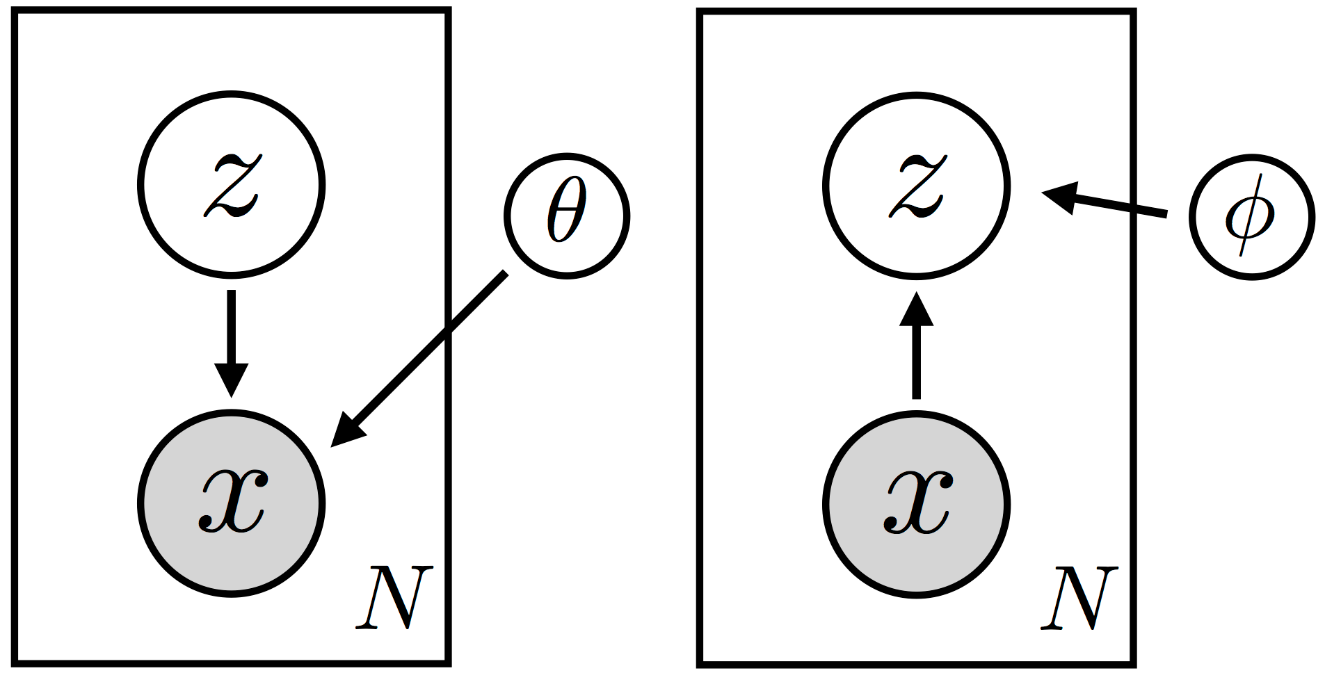
Graphical notations of a VAE encoder (on the left) and decoder (on the right).

The relation between the $x$’s and their $z$’s is parameterized by a neural network, acting as an encoder. It can be highly nonlinear and domain-specific (e.g. using sliding windows convolutions for images). The model $p_\theta(x)$ corresponds to the encoder and the posterior $p_\theta(z \mid x)$ corresponds to the associated decoder.

As above, to make the problem tractable, we surrogate the posterior probability with a deep neural network $q_\phi$. The parameter $\phi$ defines a class of distributions, in which the optimum $\phi^*$ in the KL sense is selected by training the autoencoder. This design allows to learn the guide from a dataset of observations, the supervision being provided by

• the reconstruction error on the $x$’s (MLE criterion);
• the KL divergence between the guide and the posterior (ELBO criterion).

We usually target the class of normal distributions by outputting the mean and log-standard deviation of a multivariate Gaussian law, i.e. $\phi = \{\mu, \log \sigma\}$. Once the encoder is trained together with its corresponding decoder, the associated guide $q_\phi$ fits the true posterior distributions of the latent variables as well as possible.

Note that the forward pass samples $\widehat{z}$ from $\phi$ and decodes it into a plausible observation $\widehat{x}$ with the decoder $q_\phi$. We call it a generative model as it tries to discover the true structure of causality explaining the data and not only tries to mimick it.

References

• Ulrike von Luxburg, Statistical Machine Learning (Part 12 - Risk minimization vs. probabilistic approaches), Summer Term 2020, University of Tübingen. ↪
• Pyro.ai tutorials, Variational Autoencoders. ↪
• Matt Hoffman, David M. Blei, Chong Wang, John Paisley, Stochastic Variational Inference, Journal of Machine Learning Research, 2013. ↪